
Many of us at Michaels are gluttons for data and accompanying analysis. Our homes are test beds. In this post, we look at impacts from smart thermostats, the dangers of wrong assumptions, and extrapolating findings for impact evaluation.
Every smart thermostat evaluation I’ve seen uses billing regression models to estimate savings. Unfortunately, this provides an answer and typically not one smart thermostat makers like. The evaluations typically provide no “why” to the results, and therefore, smart thermostat programs go unimproved.
Test Bed Description
My single family home was built in 1934, has crumby, double-pane, double-hung windows, and unknown amounts of wall insulation. The walls have thick plaster over heavy wire mesh that would serve any wrecking ball with a stiff challenge. The heating system is equally stout with cast iron radiators. In total, there is enough steel to build a bridge across the Mississippi. The system and structure (stucco exterior), with all its steel and contained water, is quite massive, infinitely more massive than a furnace and forced-air duct distribution.
The heating temperatures are set as follows this season.
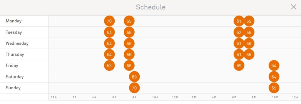
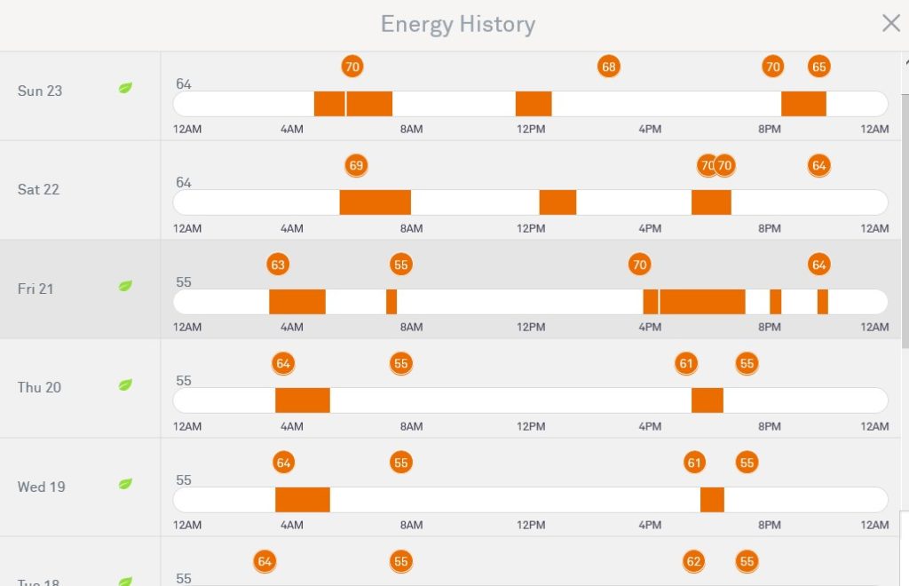
Effects of Mass
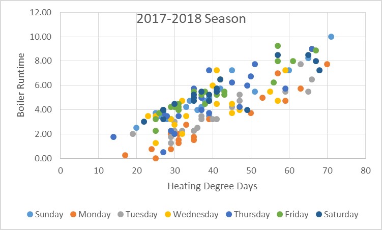
The most recent runtimes are shown in the chart below, which indicates how massive the system is. Once heated, it coasts most of the time.
We can see from the temperature schedule above that the profiles for Friday and Monday are mirrored. They both heat the space to 70F one time, so they should have similar heating requirements, right?
Wrong!
Perilous Assumptions
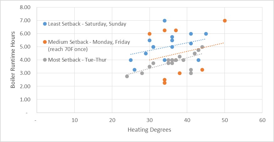
*Note, each data point represents a day. Heating degrees are described below.
On Monday, the mass of the home is warm, and therefore, it only takes a little poof of heat to bring it off night setback in the morning. The setback temperature is 65F Sunday night and 55F at the start of warmup Friday. It isn’t the set point that matters much; it is the starting conditions.
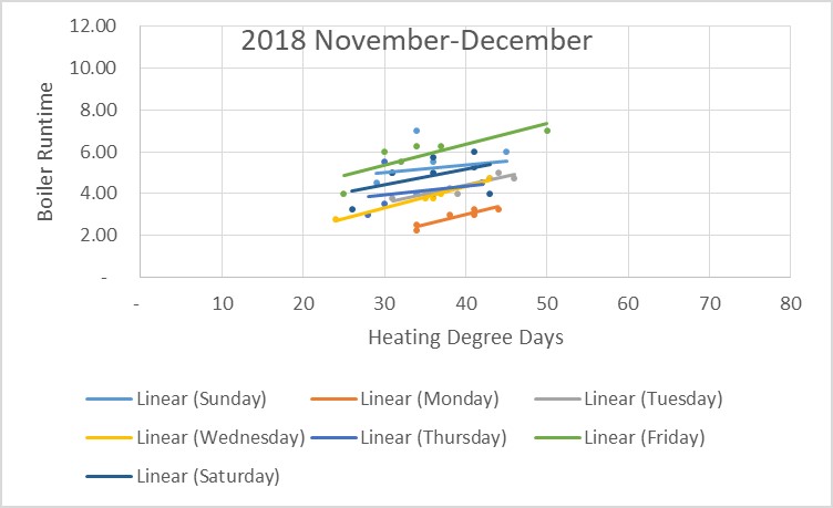
This is a lesson learned. After assuming one thing, the data reveal something else. Therefore, the next step: profiles by the day of the week – more granularity than guessing days of similar patterns. The next chart illustrates this.
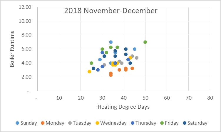
Unfortunately, thus far this season, we have not seen much variation in weather. December, when the temperatures plunge on average, has been almost as warm as November. However, for the day of the week assessment, we can clearly see the trend from day to day.
- Monday requires the least heat.
- Data for Tuesday, Wednesday, and Thursday are piled on top of one another because they have similar setpoint schedules.
- Friday, with less setback than Saturday or Sunday, represents the greatest usage due to thermal-mass effects.
- Saturday and Sunday, representing the least setback, have the most volatile gas consumption. Why? I suppose it could be rationalized by internal gains. I used the oven a few times and the TV once in a while. A candle produces more heat than my LED light bulbs.
Last year, there was substantially more scatter, shown for the entire season in the following chart.
Dangerous Extrapolations
The next couple of charts show linear fits by day of the week for this heating season to date and last year’s full heating season.
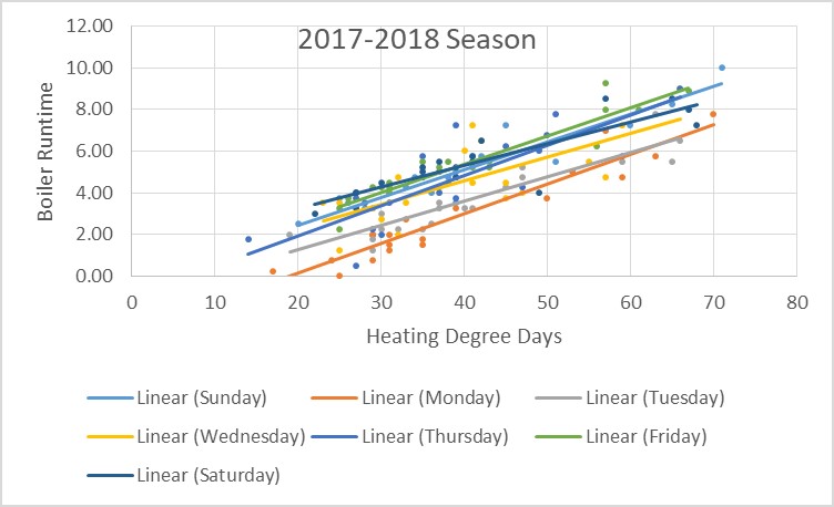
One of the many critical things we learned in college was never to extrapolate or project what would happen outside the bounds of the data set. For example, last heating season I collected data starting around the same time, early November, but by New Years, we had substantial cold weather where some average daily temperatures were below zero, which means there were more than 65 heating degrees some days.
The normal base outdoor air temperature is 65F. Let’s call this the breakeven temperature. This simply means when it is 65F outside, the home needs no heat to maintain a 70F indoor temperature. Internal gains such as electronics, lighting, cooking, and beating hearts provide enough heat to overcome the five-degree differential.
The data for both years show setback clearly saves energy, as demonstrated in the plot below. Friday has the biggest load, pulling everything out of weekday setback. I think my setbacks are less aggressive this year, and therefore, slightly more gas is used.
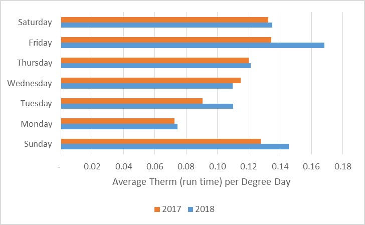
However, 2018 data are somewhat inconclusive. It may, and hopefully will, turn out to use less heat this year. Why is it inconclusive? Because when extrapolated to a full year it is certainly not fully representative. How can we tell?
Old school – print the plots and extend the curve fits with a straight edge until they cross zero. Remember, the assumption is a 65F breakeven temperature. If the indoor temperature setpoint is 55F and no one is home, guess what – the breakeven is 55F. When it’s colder than 55F outside, we need heat to keep it at 55F inside.
The breakeven temperatures are as follows.
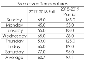
I have two months (!) of data so far this season, and it tells me my breakeven temperature is 97F on an average day. Wow! I need heat to maintain 70F until it’s 97F outdoors! Wrong! More data required. We need some cold weather and warm weather to get this squared away. I’ll come back to this in April or July if winter lasts until May again this season.
The bottom line:
- Practitioners need to be careful with data.
- Data need to be observed from multiple directions.
- Extrapolating beyond the data set is foolhardy.
- Building and system mass can be a much larger flywheel than is typically assumed.