Quirky nerd alert: fans and pumps are the lungs and heart of industrial facilities. They move air, oxygen, heat, particulates, as well as cool systems and equipment. However, unlike mammals, the lungs and hearts of industrial systems and facilities do not evolve to match their use case or be efficient.
“Efficient” is a funny word. A widget, like a pump, can be efficient, but only if it is designed into a system to operate at its sweet spot. E.g., Volvo doesn’t install the engines it uses for its commercial semi-trucks into its XC wagons. Like mammals, they are mass-produced. Industrial systems, on the other hand, are designed and built with double sets of belts and suspenders (extra capacity and power, just to be safe), and maybe some duct tape and bubble wrap. Fans and pumps and the flows they can deliver are often grossly oversized.
The Cube Law: Why a Little Extra Flow Costs a Lot of Extra Power
To give readers some mathematical background into fluid (air, water, or other gas or liquid) flow and power, here are some mathematical truths that we learned and measured in engineering school:
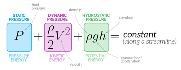
- Again, referencing the Bernoulli principle, pressure in fluid dynamics (P in Equation 1[1]), whether air, water, or some other gas or liquid, is proportional to velocity squared.
- Flow in gallons per minute (gpm) or cubic feet per minute (cfm) equals the average velocity times the cross-sectional area.
- Fluid power is proportional to the pressure times the mass flow, which is simply volume flow (cfm or gpm) times density.
- Therefore, power is proportional to velocity or flow cubed (∝V2 × V)
Equation 1 Bernoulli
How to Read a Pump Curve (and Why the Sweet Spot Matters)
I will start with a pump curve, as I worked with it a thousand times back in engineering school and on the job at Michaels Energy. NOTE: Many fan curves are quite similar, so we can learn about fans and pumps simultaneously.
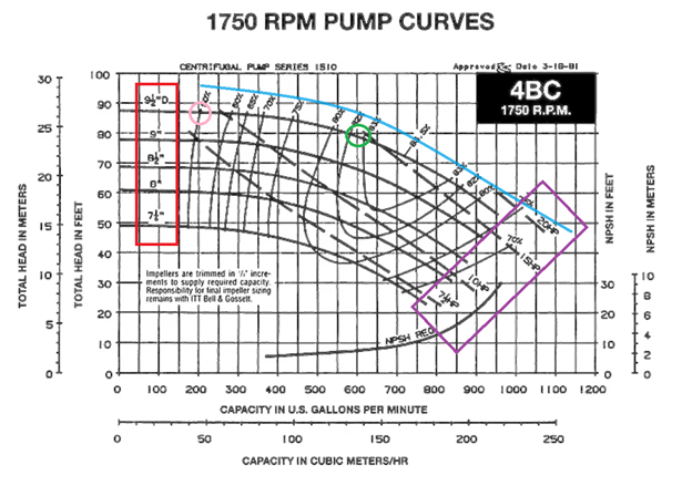
Figure 1 shows pump performance for various impeller diameters of the pump shown in the red box. The only difference is the smaller diameters, e.g., 7 ½ inches, which is a turned-down (shaved-off) version of the 9 ½-inch impeller. Pump flow (x-axis) for any of the curves produces exactly one pressure or “head” (y-axis). For example, a 9 ½-inch impeller at 600 gpm (gallons per minute) produces about 90 feet of water pressure. That operating point is in the green circle. 90 feet of water is equivalent to about 40 psig, which is close to the pressure in a car tire.
Figure 1 Typical Pump Curve
Throttling Oversized Pumps
Efficiency curves intersect the pump curves more perpendicularly. Efficiencies are shown as percentages along the blue line. The efficiency at the operating point in the green circle is about 82.5%, which is very good. But what if the pump is three times too large and the required flow is only 200 gpm? For that impeller, the flow slides back on the 9 ½” curve to the pink circle, which shows an operating efficiency of a measly 50%. Thirty percentage points of efficiency vanished. However, at least the power declined from around 15 horsepower (HP) to roughly 8 HP (dotted lines with HP numbers in the purple box.)
No Throttle, No Mercy: the Worst-Case Scenario
Therefore, if the application or the load only requires 200 gpm, it is better to throttle (waste energy) than to give the load 600 gpm, which would waste even more energy. Believe it or not, there are unregulated flow regimes out there. They might include steel mills to keep equipment, like rollers and bearings, cool, or systems with bypass, in which whatever the load doesn’t use is bypassed around the load and back to the source. As shown in these cases, the pump may be efficient, but it’s wasting lots of energy pumping water that provides no benefit to the load or process.
Minimizing Pump Energy with a Variable Frequency Drive
Actually, bypass was/is a typical control strategy for chilled water systems. A classic fix for this is to plug the bypass port or install a two-way valve (the three-way valve has a bypass port) and then control water flow with a variable-frequency drive. Then it’s really saving energy because both the flow and pressure are reduced compared to throttling (riding the curve) or full unimpeded flow with bypass.
Major Minor Losses
Engineers learn about major and minor losses in fluid dynamics class, which studies flow regimes and energy loss (essentially friction and turbulence) in piping and ductwork.
Major losses, which may not be so major, are associated with friction flow in straight pipes or ducts. Minor losses are associated with friction and turbulence due to flow disturbances, changes in direction, mixing, etc.
Pressure drop in straight pipes, fittings, and other flow disturbances, including valves, is proportional to flow or velocity squared as described above. Since flow disturbances causing minor losses involve significant turbulence, minor pressure losses are not calculated using the Bernoulli principle. Instead, they are empirically modeled and determined. The modeling results in a “k-factor” or loss coefficient for each type of disturbance. The pressure drop through the fittings and valves is proportional to the square of the flow, per Equation 2.
Equation 2 Minor Pressure Loss Equation
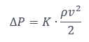
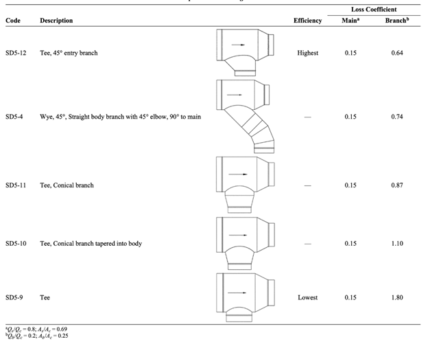
Table 1 presents loss coefficients (K) by fitting type. You can see that rounded corners can reduce pressure loss by 75%, wye versus tee by 50%, etc. Similarly, Table 2 shows minor loss coefficients for variations of tee connections for ductwork. Here, we see that pressure losses can be reduced by about 70% with gradual turning of the airflow, compared with a traditional blunt tee joint with a loss coefficient of 1.80.
Table 1 Fitting Loss Coefficient Table
Fitting Type | Description | K (Typical Range) |
90° Elbow (standard, sharp) | Short radius | 0.9 - 1.5 |
90° Elbow (long radius) | Smooth turn | 0.2 - 0.4 |
45° Elbow | Gradual turn | 0.2 - 0.4 |
Tee (flow through run) | Straight through | 0.6 - 1.0 |
Tee (branch flow) | Turning into branch | 1.0 - 2.0+ |
Wye (Y-fitting) | Gradual split/merge | 0.2 - 0.6 |
Sudden expansion | Sharp area increase | 0.5 - 1.0 |
Gradual expansion (diffuser) | Tapered | 0.1 - 0.3 |
Sudden contraction | Sharp area decrease | 0.4 - 0.8 |
Gradual Contraction | Tapered | 0.1 - 0.3 |
Fully open gate valve | Minimal restriction | ~0.1 - 0.2 |
Globe Valve (open) | High loss valve | ~6 - 10 |
Table 2 Ductwork Joint Coefficient Values
Miscellany
Lastly, I will provide an example of common sense regarding fluid flow. The Air Movement and Control Association provides an excellent article on this that illustrates exactly what I was thinking. The phrase “there’s nothing less common than common sense” comes to mind.
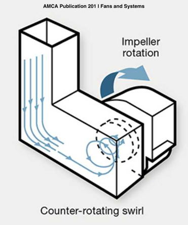
Centrifugal fans and pumps, the vast majority by type, induce fluid spin as it enters and exits the machines. If any pre- or post-swirl accommodation exists, use it, and don’t fight the flow. For example, the fan entrance shown in Figure 2 induces a counterclockwise spin while the fan is spinning clockwise. That’s wasted energy, like slamming the gas pedal to the floor to slam on the brakes at a stop light, only to speed up again.
Figure 2 Counter Spin Entrance Losses
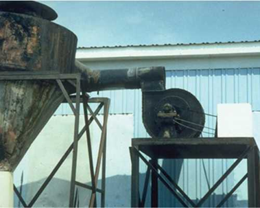
The fan and duct configuration in Figure 3 wins the engineering efficiency award for anything I’ve seen, although I have seen scenarios that are nearly as bad. Here we have counter spin, in addition to a super hard, choking left turn.
Figure 3 Counter Spin Exit Losses
The Industrial Difference
Many of the opportunities presented in this post do not financially pencil out for commercial and residential applications. However, due to industrial-facility operating hours of 24/7/300+, many measures, such as system reconfigurations and new pumps or fans, pay off in 2 years or less.
Next up: process heating systems.