Last week I related electrical demand in kW with electrical energy in kWh. Energy is the area (power times time) under the kW curve. Without cheating, I’ll do an example.
Elementary Calculus
In energy-nerd world, a curve is a line of any form, including a straight line. Consider the simple ax + b curve on the right, where a is the slope and b is the y-intercept. The equation is y = 2x +4. C’mon you had this in elementary school. Challenge yourself!
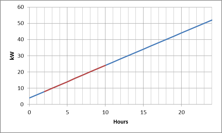
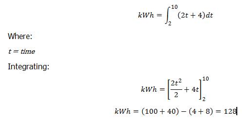
If I want the energy consumed from hour two to hour ten, I simply take the integral of this equation from two to ten:
If you remember anything about grade school geometry, you can determine the area under this line without calculus. Test your brain and see for yourself.
Cheater Calculus
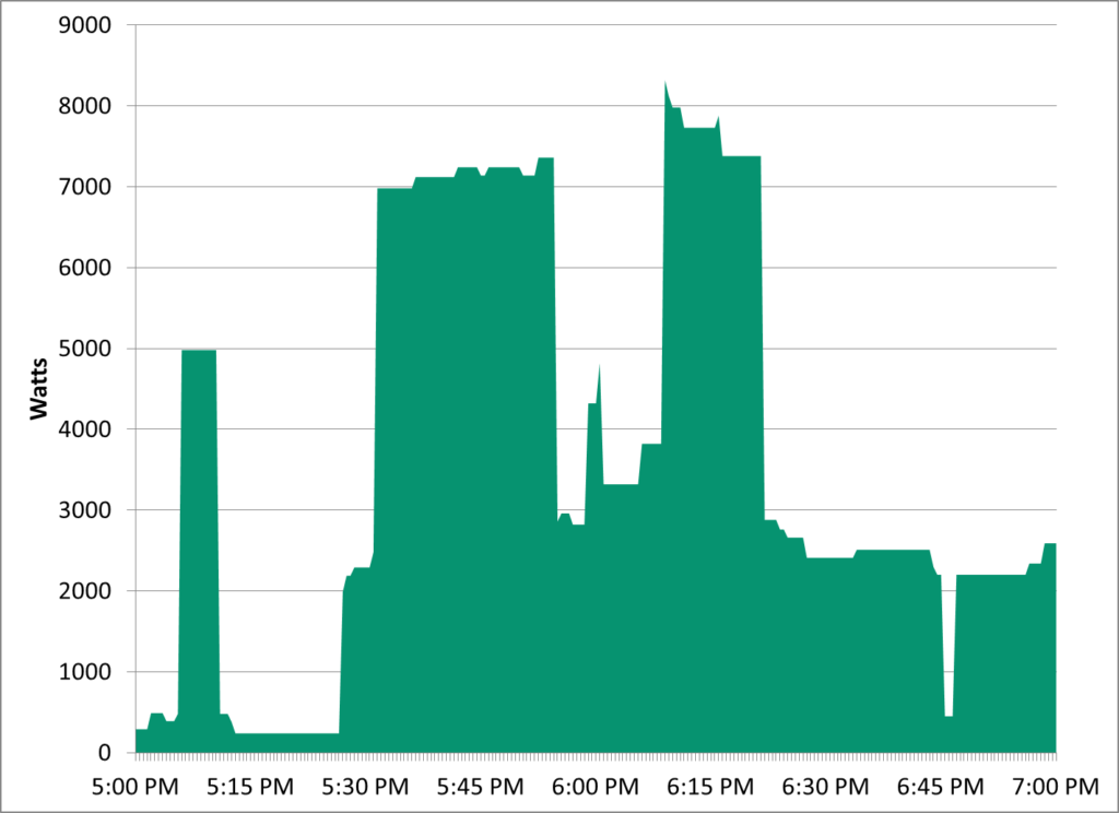
Want a cool idea for doing integration with no calculus training whatsoever? (This is what we learn in grad school, mechanical engineering) Say you have a hideous looking curve like the one in last week’s post, shown below. Without chopping that up into small pieces, you’ll never find an equation for that curve. This is not unlike something you’d experience in a lab setting. So what do you do? Get a printer and some good scissors.
See where this is going? Print two copies. Cut out the perfect square of 2 hours × 9 kW. Weigh it. This gives you kWh per microgram of paper. With the second copy, carefully cut out the green part. Weigh it. Multiply the weight of the green piece (no pun) by the calculated kWh per microgram of the 2×9. Ta dah! 7.4 kWh, right on the dot. Rip the kids away from their books and video games. This will blow their mind!
Commercial Building Demand
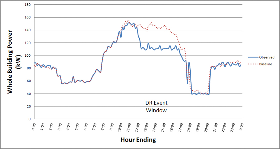
Load profiles for homes are choppy like the one shown to the right. Commercial buildings have smoother load profiles because they have more loads and steadier loads. Most of the lights are on all the time. Pumps, fans, and maybe cooling run constantly. This is demonstrated in the load profile example below from Canadian Consulting Engineer. This shows demand response, but the normal load is demonstrated by the dotted line.
Grid Level Demand
Once it all rolls up to the grid level the curves become smoother as shown in the following curves from PJM Interconnection. PJM serves the Mid-Atlantic from Virginia north to Pennsylvania and New Jersey, west through Ohio including pockets of Indiana, Michigan and Chicago. Resource capacity for the PJM region is driven by summertime cooling loads as shown in the charts.
Peak Periods
Peak periods for determining customer billed demand on a monthly basis are defined in utility tariffs. Short of an exhaustive review, peak periods are typically 12 hours, 8:00-8:00 or 9:00-9:00, Monday through Friday, minus holidays.
Billing for Demand
Demand tariffs include charges for on-peak demand. As described last week, that is the highest 15 minute integrated average during on-peak hours during the billing period. Most utilities use a sliding 15 minute window, while some use discrete periods end to end.
Some utilities bill for off-peak demand if it exceeds on-peak demand. The charge is usually, if not always, less per kW than on-peak demand.
Most demand tariffs have a “ratchet” clause; a lousy term, like the alternative minimum tax, which is actually an alternative maximum tax. This should be called the alternative maximum demand. The clause typically reads that billed demand shall not be less than 75% (or 50% or some other number) of the maximum peak demand in the previous 11 billing cycles.
The objective of demand billing is equity. Utilities build infrastructure (rate base) for the maximum load on the system. It could be argued that everything but the fuel used is a fixed cost and therefore nearly the entire bill is demand charge. The cost for meeting peak loads is the cost of rate base or maintaining the rate base. Indeed, some tariffs charge a lot for demand and practically give energy away.
Coincident Peak Demand
Customer peak demand can happen anytime 24/7. Customer on-peak demand can happen anytime between 9:00 and 9:00, M-F. Coincident peak demand is the customer’s demand during the grid’s peak hours, which as shown in the PJM charts above is generally three to four hours that include 5:00 PM, M-F. Many times for EE programs, regulators and independent system operators (if they buy demand side resources) want to know the coincident peak demand savings of each measure. This saves ratepayers by delaying or avoiding added supply-side resources.
If the coincident peak period is only three or four hours per day, why is the on-peak period twelve hours per day? Coincident peaks are when the generating assets are approaching full capacity across the grid, except renewables, especially wind, which is unreliable.
Generating capacity is often not the primary constraint. The primary constraint can be a stressed substation or feeder. A feeder is a power line that provides electricity to customers in one direction. If the loads on that feeder become excessive, the voltage drops outside of specified levels, causing problems for some customer equipment. The peak period on a feeder could be completely different than the coincident peak.
Therefore, it can easily be argued that programs targeting the most stressed substations and feeders are a better solution. Pilots are already underway.


Join the discussion One Comment