In recent years, there has been a push by some intervenors and program implementers to move larger and larger, and riskier measures from custom efficiency into prescriptive buckets. These include air handling system replacements, control system replacements, and of course, the variable frequency drive.
To make sure everyone is on board, prescriptive [incentive] savings are determined for a specific piece of equipment, or determined by preset formulae with some combination of stipulated (assumed) values and project-specific information. This is opposed to custom savings calculations that are estimated by an engineer/philosopher according to the project specific application.
Uncertainty
If there are two classes of widely adopted projects or technologies that rise to the top of uncertainty and magnitude of savings, they are variable frequency drives and compressed air anything.
Why?
Because nobody knows how the existing equipment operates or is controlled or what load factors are. A load factor is percent loaded, or percent power. A truck [engine] pulling a load up a long hill is near 100% load. A car zipping past the truck might only be 60% loaded. I, or anyone else, can tell the truck is fully loaded. No one knows about the car. The same goes for pumps, fans, and air compressors. But this is only one piece of the puzzle.
Research
For variable frequency drives (VFDs), we polled a bunch of technical reference manuals (TRMs) and other deemed savings sources to compare and contrast methodologies. These include eight statewide TRMs and algorithms from three investor-owned utilities (see summary of findings here).
To my surprise, as many as eleven different approaches to determining savings for variable frequency drives exist; these go to every corner of the universe.
Key Findings
- Eligibility for prescriptive VFDs varies widely from HVAC pumps and fans only, to practically anything.
- The connected load or motor/drive horsepower limits vary dramatically from an upper limit of 10 hp to an upper limit of ∞ (no limit).
- Algorithms are all over the place from a two-parameter lookup table to formulas with several project-specific inputs to be provided by trade allies.
- Accounting for application types, building types in particular varied greatly from nothing (one option) to at least a dozen. Specifying equipment varied from fans or pumps (two options) to multiple fan and pump specifics based on existing control (up to ten options).
- Only one addressed what to do for installations on backup or standby equipment.
- Only a few mentioned that automatic controls were required.
Discussion
Rigor and Precision – Haha, it is to Laugh
Example: You need to measure the dimensions of your garage to put down a floor sealer. What do you do? Most people would go for their tape measure. Nerds would get their laser measuring device.
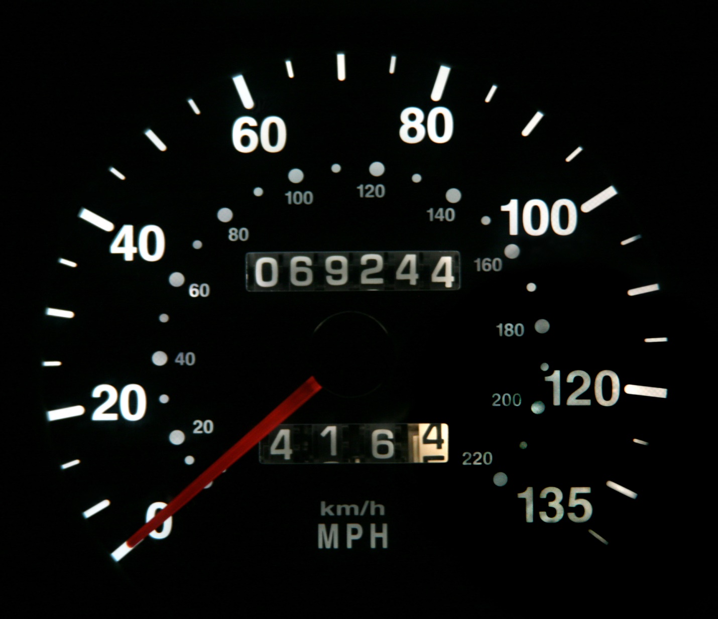
Back in the day, we had mechanical odometers like the following. Without a custom calculation by a decent engineer, you might as well guess the garage dimensions without ever seeing it. Otherwise, it would be like measuring the garage with an old-fashioned odometer. The theory is wonderful and defendable, but trying to collect data accurately from market actors and calculating something is a fool’s game. I understand we need some accurate-looking all-inclusive algorithms and calculations behind it, but I wouldn’t buy any of it without my own back of the napkin calculation.
Controls
All serious Rant readers know control is everything. It’s the difference between getting savings for installing a smart thermostat and whether or not it is connected to anything. And believe me, we have seen new thermostats on the wall and not connected to anything.
Impact Variability
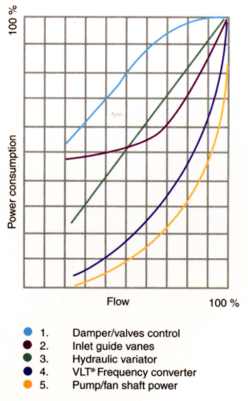
The chart below is a typical set of power curves for various control types. Variable frequency drives are represented by the blue curve, which rides just above the yellow curve, which represents power delivered to the shaft impeller/wheel of the pump/fan at varying speeds. Not shown is bypass or full flow, which is 100% all the time. Bypass and full flow are not uncommon. Applications include smaller fan systems, chilled water systems and cooling water systems.
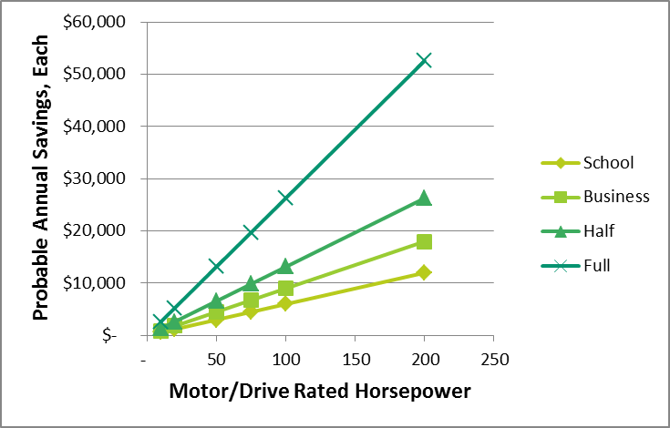
How might annual savings look for different applications? This is shown on the next chart. These are for typical hours for the applications shown. Half and full is simply half the hours, and all the hours of the year, respectively. This could represent a hospital or part time manufacturing, and full time manufacturing.
Not mentioned yet is the fact that many pumping systems have full backup capability, consisting of two pumps piped in parallel. It is easy to get rebates representing twice the actual savings for such a case because one is always de-energized.
Conclusion
This mini-study actually leaves me with a compromise. I had thought a custom approach should be applied to applications as low as 20 hp. Indeed one state shown above goes as low as 10 hp. For equity and fairness reasons, my recommendation is 50 hp. This size application would generate impacts in the $3,000-$15,000 range and as a percentage, engineering costs for custom calculations are low.
Why does it matter?
The vast majority of energy savings that flow through prescriptive programs have a linear uncertainty – that is, savings vary mainly with hours per year. Power savings are known quite confidently, and therefore energy savings is merely a matter of run time. You can see from the percent flow/power chart for drives above that power saved can be zero to 90%, times run time – which too is zero for standby equipment. There are no standby light fixtures.